I have always wanted to "get into" machine learning, but I was always overwhelmed by the vast number of libraries, backends, and packages there are. I learn a lot by the implementation of something, much more so than just reading the math that describes the behavior.

This last semester of my masters degree, I am taking a deep learning course. Although this course isn't focusing on implementation of algorithms primarily, I am planning on following along with implementation in Julia.

I have gotten pretty far already, and I have learned SO much more in doing so than what I have gotten out of the class so far. I wanted to document this process for anyone who is in a similar place and wants to learn more about using Julia for machine learning.

Tooling

I made a decision early that I wanted to write most of the code for this myself. I didn't want to use TensorFlow, Keras, or whatever. This is because I am not interested in learning a tool, but rather learning how the tools work. I believe that if I understand this, then using the various tools will come later. I end up using one Julia package, but I will explain why in a bit. The machine learning library Flux.jl claims that I could have written it all myself so might as well try.

And we're off!

So in the class we started with gradient descent. I'm not going to go into the details here as there are a multitude of resources online to learn, but I will discuss my implementation. I wanted my code to be as generic as possible and as such each model will be composed of a struct and a (C++ like) functor.

For example, if my "model" was a line, I would write it like this:

struct Line
    m
    b
end
(l::Line)(x::Real) = l.m[1]*x + l.b[1]

So, given a "Line" object, it is callable with some input "x". This is a nice pattern as I can have a struct that encapsulates the parameters of a model and a functor that uses those parameters to define some behavior. I have "m" and "b" as vectors because the Line struct is immutable and multi-parameter models will have their parameters as vectors as well in the future, so I just want to be consistent here.

Next on the docket was generating some random linear data to fit. I did so simply like this:

x = 1:100
y = @. 3x + 100 + 100*rand()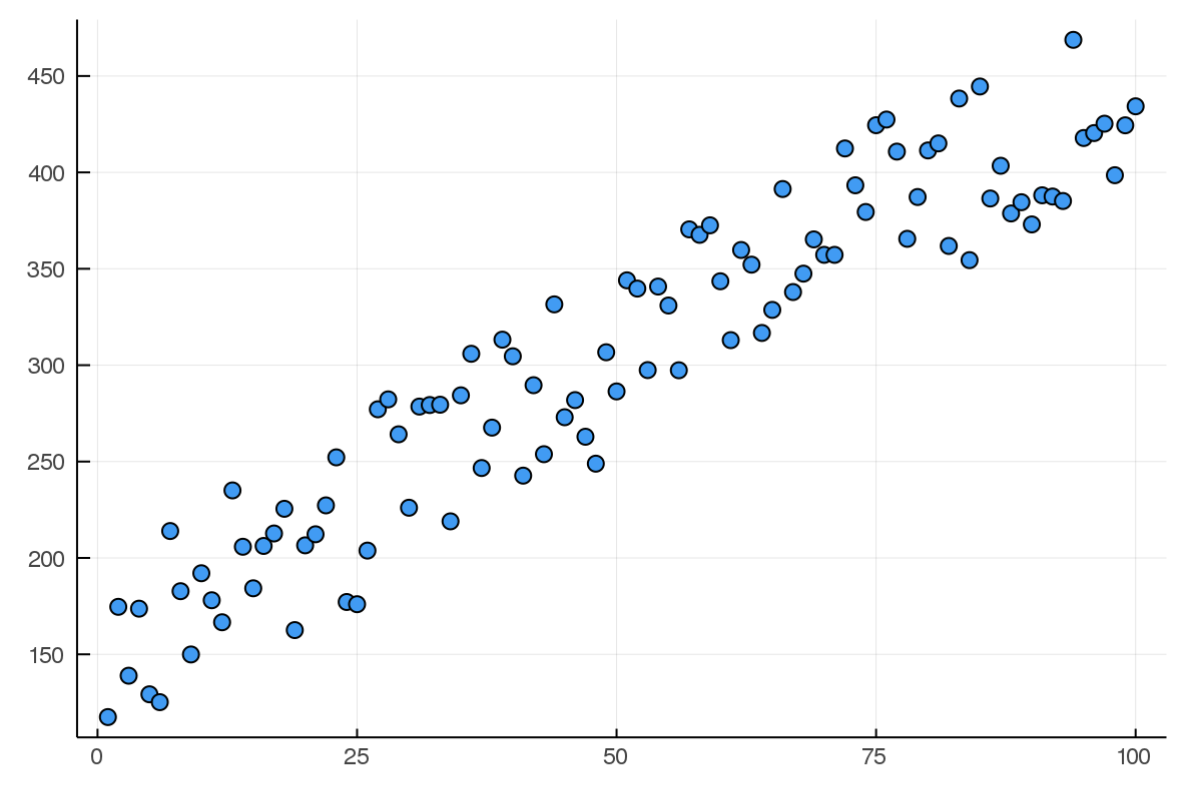

So far so good, now we need a function that will act as our cost; how bad is our assumption? As we used mean squared error in class, I will just be using that, easy peasy. I'm using the dot broadcasting syntax here to apply the square error for EVERY term in y and ŷ as we want to calculate this error over the entire model, which will be a vector of guesses and correct outcomes.

mse(y,ŷ) = (1/length(y)) * sum((y-ŷ).^2)

Now, we have two more functions to write. One will be our main training loop and one will be the gradient descent code. As I want my training code to be as generic as possible, the training function will take in the "optimization" function as an argument, so I can write other optimizers in the future and not have to adjust the training loop.

So this is where things get tricky I need the gradients of the loss function given an arbitrary model. I can start by looking how I calculate this loss over the model. If I start with a randomly initialized model, I can broadcast that model's functor over the input data set and feed that into the loss function.

Line() = Line([rand()],[rand()])
model = Line()
totalCost = mse(model.(x),y)

For this randomly initialized line model, my total cost was around 86000. The goal now is to adjust m and b such that cost is minimized.

Gradient descent describes a certain "update rule" that given the partial derivatives of each model parameter for the total loss, we just update each parameter with that gradient times some arbitrary learning rate α. Here is where I leverage another package for help. One of the reasons Julia is awesome is because of the simple and powerful Automatic Differentiation engines it has to offer. If you haven't already, watch this video. It shows how easily such an engine could be written in Julia. I am choosing not to write this as I want to focus of the ML algorithms and not the gradient algorithms. This makes sense to me as I could write an AD engine, but most of what I read about ML assumes you already have the gradient available. Additionally, now this idea of using arbitrary model structs and functors can be plug and play and the gradient will be calculated exactly in the background. I am using Zygote as my AD engine, it seems to be the most fleshed-out right now, but there are several out there to choose from.

Take our line model for example. Using Zygote, I can just call this function to get those gradients I described.

g = gradient(model->mse(model.(x),y), model)

Without telling Zygote how the mse function worked, or how that model functor behaves, I got a named tuple result of the gradient:

((m = [-32761.03206258861], b = [-566.5599674909674]),)

Just like that. It's exact, its fast, its flexible, and I don't see any reason not to use this.

So now given this gradient, I can write my update function. This gets a little metaprogram-y as I have to query the fields of the struct so I know what to update if there is a better way of doing this, let me know. I'll walk through this line by line.

function gradientDescent(model,g;α=0.0001)
    for field in fieldnames(typeof(model))
        broadcast!(-,getproperty(model,field),getproperty(model,field),α*g[field])
    end
end

So this function takes a model, the gradients of the model, and that learning rate term α. I then iterate through all the fields of the model. So each field will be a symbol from the type of the model, in this case field will be :m and :b. Finally, this is the weird line, I use the mutating broadcast function to assign each field in the model to itself α \* the gradient of that parameter. This is equivalent to saying model.field -= α \* gradient. I can't use the dot syntax here as the field variable is an unresolved symbol.

Finally, I write a train function that takes all this in and iterates until some convergence.

function train!(model,inputs,outputs,N,cost,optim,conv;kwargs...)
    costs = [cost(model.(inputs),outputs)]
    for _ in 2:N
        g = gradient(model->cost(model.(inputs),y), model)[1]
        optim(model,g;kwargs...)
        push!(costs,cost(model.(inputs),outputs))
        if (costs[end-1] - costs[end]) <= conv
            break
        end
    end
    return costs
end
train!(model,x,y,100000,mse,gradientDescent,eps(),α=0.0001)

Once again, line by line: my train function (mutating the model in-place, hence the bang), accepts a model, an input vector, and output vector to train against, N iterations, a cost function, an optimization function, a convergence criteria, and various kwargs we can pass around. I start by initializing a vector of costs per iteration with the initial model cost, then iterate through my optimization step by calculating the gradients and passing them to my optimizer. If i reach convergence, I break early. I call this train function with my model, the training data we have, the mean squared error cost function, the gradientDescent optimizer, and convergence I just left at epsilon to see how good it will get after 10000 iterations.

And guess what, it works!

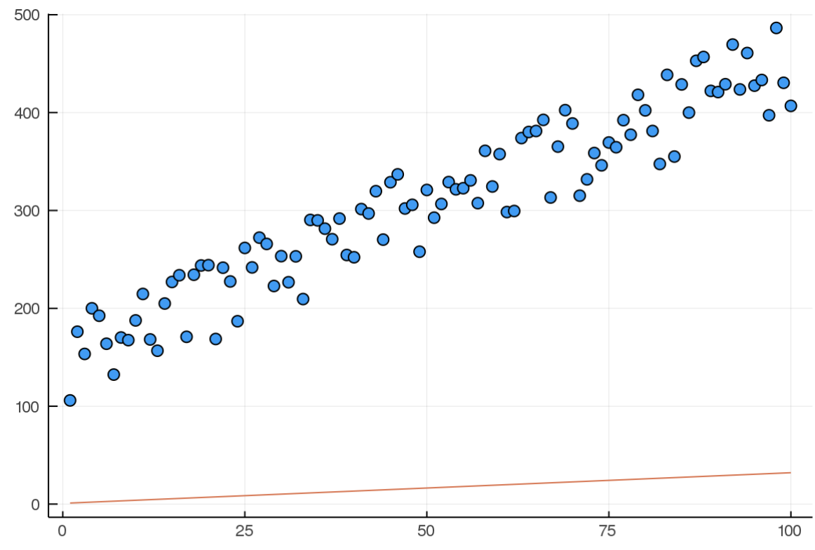
Here is the model at the beginning of training(random):

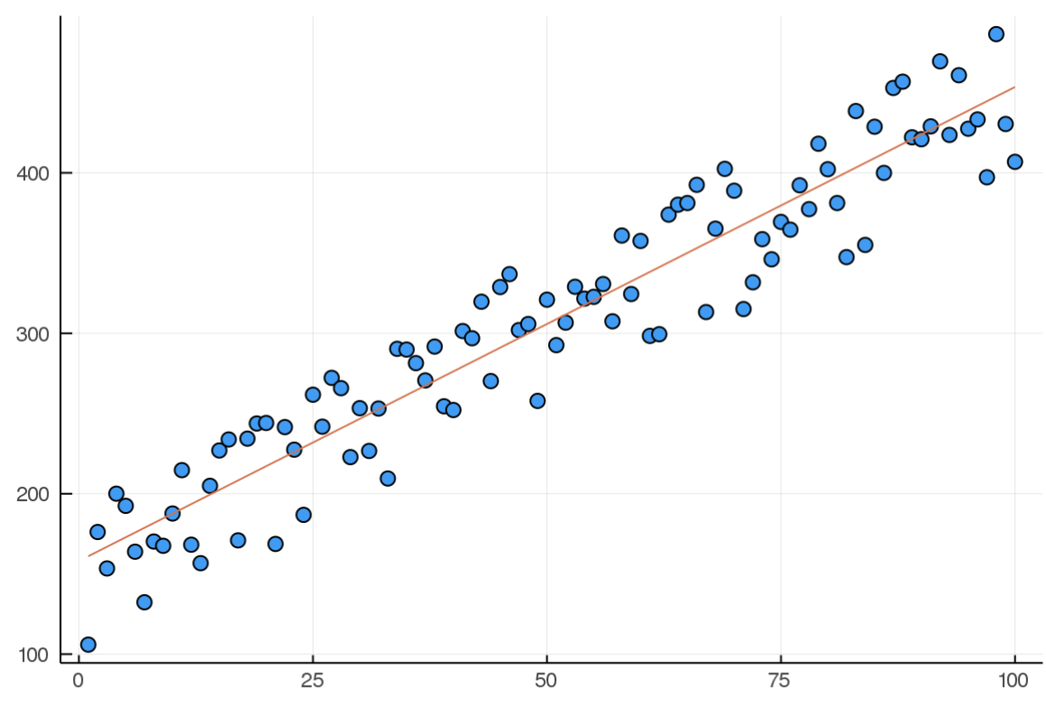
And here it is after 10000 iterations:

A few takeaways

So all in all, this was a success. In very few lines of code, I get a pretty robust gradient descent implementation. I ran into some issues with the learning rate, as a high value can make it explode. It took a while to find a good value. Here are the cost outputs from a few different learning rates:

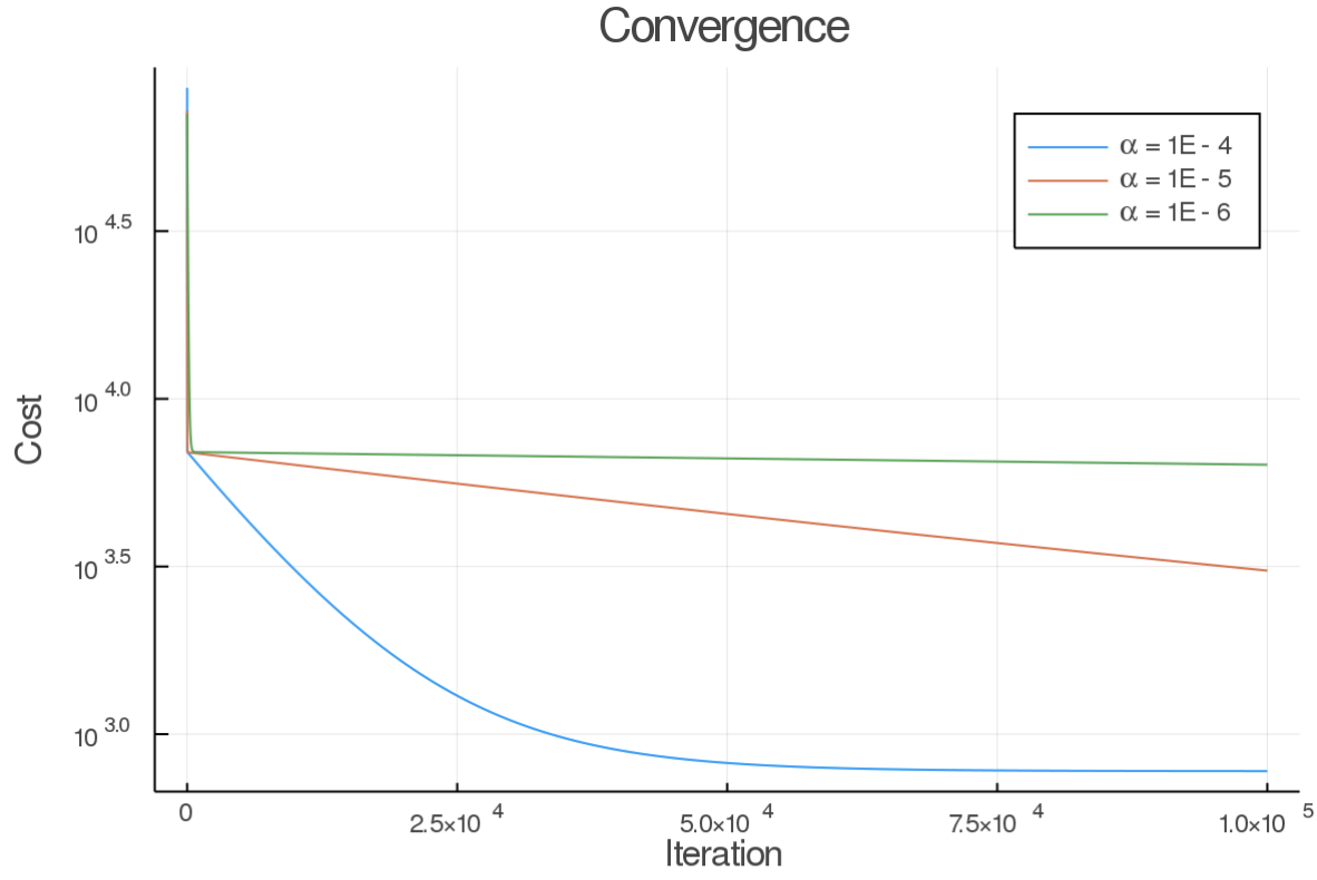
Also, the keen reader will notice that there is a period of fast convergence, and then it dramatically slows down (at least for the high learning rate). This makes sense as the learning rate is applied to both parameters, but the amount of change required for "m" is much less than is required for "b". This is evident in the cost surface. As this model only has two parameters, we can easily view it in 3D.

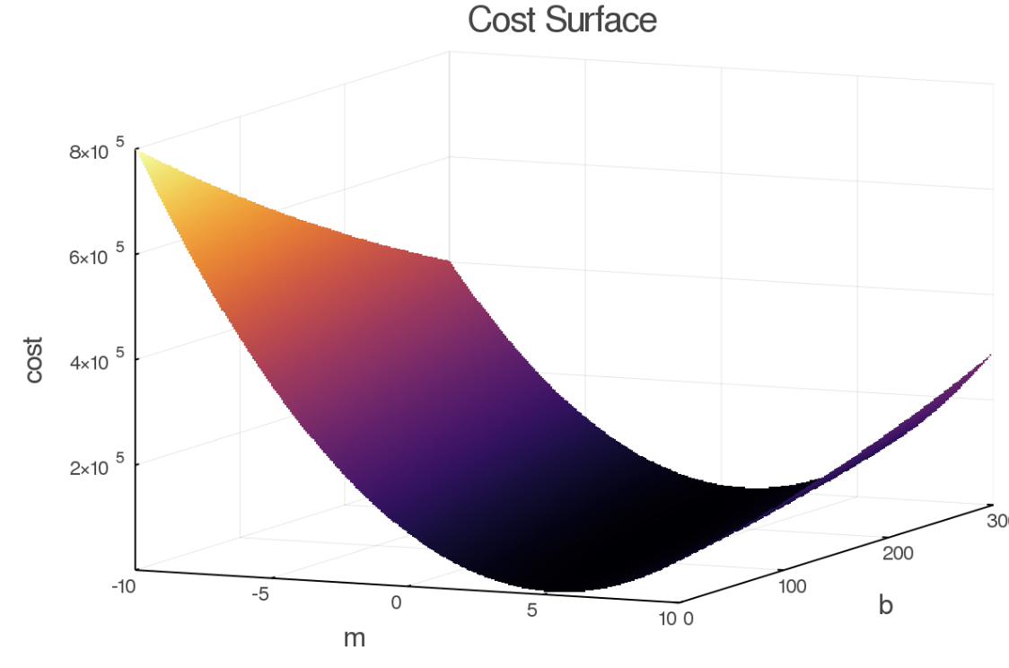
As you can see the gradient along b is generally much less than on m. This hints at some better optimization algorithms, specifically some way of choosing a learning rate PER parameter versus some global learning rate as in this case we would have wanted to take different sized "steps" in b than in m.

The beauty of generic code

As everything up to this point was generic, if I have data that would be best suited for a different type of model, I just write that struct and functor and everything else is the same. Check it out:

# New Parabola Model Parameter Struct
struct Parabola
    a
    b
    c
end
# Parabola functor to describe model behavior
(p::Parabola)(x::Real) = p.a[1]*x^2 + p.b[1]*x + p.c[1]
# Default constructor with random values
Parabola() = Parabola([rand()],[rand()],[rand()])
# Sample training data
x = -10:0.1:10
y = @. 5x^2 + 10x + 3 + 100*rand()
# Create a new random model
model = Parabola()
# Train!
train!(model,x,y,100000,mse,gradientDescent,eps(),α=0.0001)

Here is the model and training data at the beginning (random):

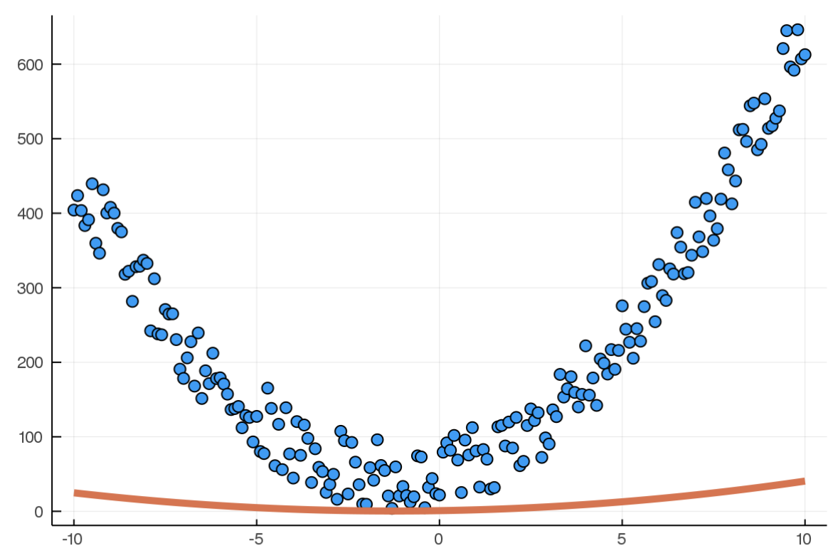
And after training

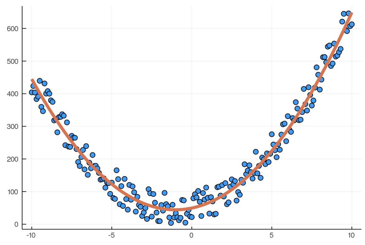
As long as I describe the model in this same way, and write a loss function that accepts the model's output and training data, everything just works! Pretty cool, right?

Up next

I have a series of posts I want to make out of this, as I actually have come a pretty long way since I started this project, I just forgot to blog about it along the way. The next post will be modifying this code to enable "stochastic gradient descent" and a look at some more complicated models (classification). I have code now written up to a fully-connected neural net and some modern momentum-based optimizers, all based on the groundwork I started here. So stay tuned!