A Finite Difference Frequency Domain Solver in Julia
There are many commercial solutions to solving Maxwell's Equations for complex electromagnetics problems. This general purpose approach is great for commercial solvers, but doesn't easily lend itself to specific problems for which a solver could be tailored for. There are a few open-source electromagnetics solvers, but the powerful of which are written in syntactically dense C or C++. For this project, I wanted to explore the simulation of a frequency-selective device, or FSS. Specifically, a binary-diffraction grating for mm-wave. These type of devices are well suited for simulation in the frequency domain. For the time being, I chose to stick with the traditional finite-difference method of solving the PDEs. So, presented in this text is a finite difference frequency domain solver using the modern programming language Julia. The device I am simulating is generalized to a 2D solution with periodic boundary conditions but could be easily extended to 3D.
What is Julia
In the realm of scientific programming, C and FORTRAN has long reigned supreme. These languages, while known for their speed, are not however known for their ease of use or approachable syntax. More "modern" languages like Python or R (to a degree) have attempted to fix the latter of the issues by purposefully compromising some performance for accessibility. This then leaves two camps of programmers, those who can't sacrifice speed and program in something archaic and those who want to be more modern. This is called the "two language problem" - the exact problem the Julia language is trying to solve.
Julia is a high-level, general purpose dynamic programming language that "looks like Python and runs like C". It is meant to provide the performance of low level languages like C and FORTRAN with the readability and expressiveness of Python. Python itself has tried to add performance through packages like numpy, by sacrifice syntax.

In many cases, Julia is just as fast as C, as seen in these benchmarks. Due to its performance, many scientific computing communities have embraced Julia for high-performance projects. The astronomy project Celeste.jl that characterizes stars brought Julia into the "petaflop club" by running at over a petaflop per second in computation.Regier:2015:CVI:3045118.3045341
As of August of 2018, Julia is in its first general release making now the perfect time to start working on large-scale projects. This release marks the first long-term state of the language in terms of syntax, style, and packages.
All of this is why I have chosen to write the code to solve the finite difference frequency domain problem in Julia. I believe with Julia, this code can be fast, efficient, portable, readable, and extensible. I am excited to continue work with Julia and I hope to contribute to the Julia project through my time working in it.
The Problem Setup
Solving electromagnetics problems is primarily a partial differential aligneds problem. Here are Maxwell's Equations in the frequency domain
$$\begin{aligned} \nabla \times \vec{E} &= -j \omega \vec{B} & \nabla \cdot \vec{D} &= \rho_v \\ \nabla \times \vec{H} &= \vec{J} + j \omega \vec{D} & \nabla \cdot \vec{B} &= 0 \\ \vec{D} &= \epsilon \vec{E} & \vec{B} &= \mu \vec{H} \end{aligned}$$Simple problems like dipole antennas and dielectric spheres can be solved analytically, but complex geometry and large-scale problems require numerical methods to solve. Lucky for us, discrete problems can be boiled down to linear algebra problems - for which we have a large arsenal of techniques to utilize.
Linear Operations as Matrices
For our case, we are looking at the differential form of Maxwell's Equations. The linear operation of interest is of course the derivative. Consider the following:
$$\begin{aligned} \frac{1}{2\Delta x} \begin{bmatrix} 0 & 1 & 0 & 0 & \dots & 0 \\ -1 & 0 & 1 & 0 & \dots & 0 \\ 0 & -1 & 0 & 1 & \dots & 0 \\ \vdots & \vdots & \vdots & \vdots & \ddots & \vdots \\ 0 & 0 & 0 & 0 & \dots & 0 \end{bmatrix} \begin{bmatrix} f_1 \\ f_2 \\ f_3 \\ \vdots \\ f_n \end{bmatrix} = \frac{1}{2\Delta x} \begin{bmatrix} f_2-f_0\\ f_3-f_1 \\ f_4-f_2 \\ \vdots \\ f_{n+1}-f_{n-1} \end{bmatrix} \end{aligned}$$Performing the matrix multiplication yields a vector of an approximation of a partial derivative of f(x).
$$\begin{aligned} \frac{\delta}{\delta x} f(x) \rightarrow \pmb{D}_1^x f \end{aligned}$$As the x spacing approaches 0, this operation approaches a perfect derivative. Because the slope is being taken at the center point of the two samples, this is a central finite difference.
One could readily write these matrices for any linear function. Fourier transforms, laplace transforms, integrals, etc. can all be approximated as a linear sum of known point of that function.
$$\begin{aligned} \pmb{L}\{f\} &\cong \sum_i f_ia_i \end{aligned}$$Constructing a complex function is then just the left-multiplication of all of these function matrices in their order of operations. Take for example the second order partial derivative. From calculus, one could simply derive twice. This is just the multiplication of two derivative matrices.
$$\begin{aligned} \pmb{D}_2^xf=\pmb{D}_1^x \pmb{D}_1^xf \end{aligned}$$What makes all of this cool is that we can reduce the entire solution space to a single problem
The Ax=b problem
Take an arbitrary partial differential aligned
$$\begin{aligned} a(x)\frac{\delta^2}{\delta x^2}f(x) + \gamma b(x) \frac{\delta}{\delta x}f(x) + c(x)f(x) &= g(x) \end{aligned}$$Term by term, the aligned can be re-written in a discrete system using matrices.
$$\begin{aligned} [A][D^1_x][D^1_x][f] + \gamma [B] [D^1_x][f] + [C][f] &= [g] \end{aligned}$$Combining like terms, we can construct an operator matrix L and simplify the problem.
$$\begin{aligned} [L] &= [A][D^1_x][D^1_x] + \gamma [B] [D^1_x] + [C] \end{aligned}$$The problem then becomes
$$\begin{aligned} [L][f] &= [g] \end{aligned}$$Programatically, all that is left is an inverse to solve for f. This is the form of the famous problem Ax=b. A is some problem, b is the "excitation" vector, and x is the solution. Simply find the inverse of A and multiply it by b to get x.
Solving in Julia
As before, Julia is meant to be a solution to fast computation with an approachable syntax. Looking at Ax=b is the perfect introduction to working with matrices in Julia.
Let's define a matrix A
$$\begin{aligned} A = \begin{bmatrix} 1 & 2 & 3\\ 4 & 5 & 6 \\ 7 & 8 & 0 \end{bmatrix} \end{aligned}$$In Julia, we would write this as the following
julia> A = [1 2 3;4 5 6; 7 8 0]
3×3 Array{Int64,2}:
 1  2  3
 4  5  6
 7  8  0
The syntax is similar to Matlab, and the result is easily understood. A is the matrix with those given entries. After we assign A to those values, the REPL returns A. Returning A prints what A is; in this case, A is a 3x3 Array composed of 2 dimensional 64 bit integers.
Making a source vector b is the same procedure
julia> b = [1;2;3]
3-element Array{Int64,1}:
 1
 2
 3
Finally, just as before, we multiply b by the inverse of A to solve for x
julia> x = A^-1*b
3-element Array{Float64,1}:
 -0.3333333333333333
  0.6666666666666666
  0.0
Simple stuff. We'll come back to this later when we start to construct the problem for FDFD.
Boundary Conditions
We left out one major talking point when discussing the finite difference method with matrices. In our derivative matrix, we included points for our function that were not in the problem space. Namely, f(0) and f(n+1). This is the boundary condition problem. As we want as many solution points as we have problem points, we have to make an assumption about how the function behaves outside the solution space. This would normally involve a long discussion about all of the different boundary conditions for PDEs, but for this implementation, we only focus on the Dirichlet boundary condition and the Floquet-Bloch boundary condition.
Dirichlet Boundary Condition
The Dirichlet condition is the most simple. In essence, for an ODE
$$\begin{aligned} y''+y'=0 \end{aligned}$$Or a PDE
$$\begin{aligned} \nabla^2y+y=0 \end{aligned}$$On the interval
$$\begin{aligned} y(a) &= \alpha \\ y(b) &= \beta \end{aligned}$$This allows us to directly assign numbers to the boundary conditions. To even further simplify this for our case, we will set alpha and beta to 0.
Floquet-Bloch Boundary Condition
The second boundary condition we will use is the Floquet-Bloch condition. This condition is used when modeling periodic devices like lattice structures, frequency-selective surfaces, and diffraction gratings. We can simulate this periodicity by equating the solution at the edges, say d(f_n) = d(f_1). Bloch's theorem states that "Waves in a periodic structure take on the same symmetry and periodicity as the structure itself."
$$\begin{aligned} \vec{E}(\vec{r}) = \vec{A}(\vec{r})e^{j\vec{\beta}\cdot \vec{r}} \end{aligned}$$Where the overall E field equals some periodic envelope that is of same periodicity as the device A and the plane wave phase tilt.
This gives a problem, though. The phase of the solution at the boundary isn't necessarily consistent. We can adjust this by acknowledging the fact that periodic solutions have the same periodicity as the device itself.
Consider the following
$$\begin{aligned} E_1 &= A_1e^{j\beta x}\\ E_n &= A_ne^{j\beta x} \end{aligned}$$But from Bloch we know the A terms are equal. so we can solve for the A
$$\begin{aligned} A_1 &= E_1^{-j\beta x_1} \\ E_n &= (E_1^{-j\beta x_1})e^{j\beta x_n} \\ E_n &= E_1e^{j\beta (x_n-x_1)} \end{aligned}$$As for this xn-x1 is the size of the space in x, we can denote it as a Lambda x. Finally
$$\begin{aligned} E_{n} = E_{1}e^{j\beta\Lambda_x} \end{aligned}$$
Frequency-Domain Maxwell's Equations as Matrices and the Yee Grid
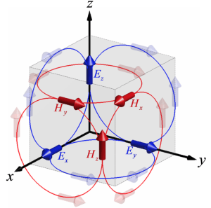
Given a discrete solution space as defined by matrices of material properties $\varepsilon$ and $\mu$, we need a method of defining electric and magnetic fields in this space. Using the “Yee Cube”Kane_Yee_1966 as shown below, we can define an electric and magnetic field for each basis of the cube.
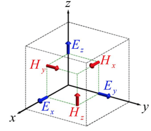
Using this cube to discretize our space allows us to easily formulate boundary conditions as well as approximate curl aligneds. Additionally, we can retain material tensors for each basis of the Yee Grid to allow for anisotropicity. There are few reasons why we use a grid of Yee cubes in a "Yee Grid"
- It's divergence free
- The boundary conditions make a lot of sense
- We can write decent curl approximations
This last one is the most important as we use the curl aligneds in solving Maxwell's Equations
Formulating Maxwell's aligneds with finite-difference is then rather straightforward. We add simplifications by normalizing with the wave number at the frequency of interest to absorb it into the spatial derivative.
$$\begin{aligned} x' &= k_0x \\ y' &= k_0y \\ z' &= k_0z \end{aligned}$$We can then easily write Maxwell's Equations as finite difference aligneds
$$\begin{aligned} \frac{\delta E_z}{\delta y'} - \frac{\delta E_y}{\delta z'} &= \mu_{xx}\tilde{H}_x & \frac{\delta E_z^{i,j+1,k} - \delta E_z^{i,j,k}}{\delta y'} - \frac{\delta E_y^{i,j,k+1} - \delta E_y^{i,j,k}}{\delta z'} &= \mu_{xx}^{i,j,k}\tilde{H}_x^{i,j,k} \\ \frac{\delta E_x}{\delta z'} - \frac{\delta E_z}{\delta x'} &= \mu_{yy}\tilde{H}_y & \frac{\delta E_x^{i,j+1,k} - \delta E_x^{i,j,k}}{\delta z'} - \frac{\delta E_z^{i,j,k+1} - \delta E_z^{i,j,k}}{\delta x'} &= \mu_{yy}^{i,j,k}\tilde{H}_y^{i,j,k} \\ \frac{\delta E_y}{\delta x'} - \frac{\delta E_x}{\delta y'} &= \mu_{zz}\tilde{H}_z & \frac{\delta E_y^{i,j+1,k} - \delta E_y^{i,j,k}}{\delta x'} - \frac{\delta E_x^{i,j,k+1} - \delta E_x^{i,j,k}}{\delta y} &= \mu_{zz}^{i,j,k}\tilde{H}_z^{i,j,k} \\ \\ \frac{\delta H_z}{\delta y'} - \frac{\delta H_y}{\delta z'} &= \epsilon_{xx}\tilde{E}_x & \frac{\delta H_z^{i,j+1,k} - \delta H_z^{i,j,k}}{\delta y'} - \frac{\delta H_y^{i,j,k+1} - \delta H_y^{i,j,k}}{\delta z'} &= \epsilon_{xx}^{i,j,k}\tilde{E}_x^{i,j,k} \\ \frac{\delta H_x}{\delta z'} - \frac{\delta H_z}{\delta x'} &= \epsilon_{yy}\tilde{E}_y & \frac{\delta H_x^{i,j+1,k} - \delta H_x^{i,j,k}}{\delta z'} - \frac{\delta H_z^{i,j,k+1} - \delta H_z^{i,j,k}}{\delta x'} &= \epsilon_{yy}^{i,j,k}\tilde{E}_y^{i,j,k} \\ \frac{\delta H_y}{\delta x'} - \frac{\delta H_x}{\delta y'} &= \epsilon_{zz}\tilde{E}_z & \frac{\delta H_y^{i,j+1,k} - \delta H_y^{i,j,k}}{\delta x'} - \frac{\delta H_x^{i,j,k+1} - \delta H_x^{i,j,k}}{\delta y} &= \epsilon_{zz}^{i,j,k}\tilde{E}_z^{i,j,k} \\ \\ \end{aligned}$$Doing this in Julia is rather straightforward. We create diagonal entries just like in the example of the 2nd order finite difference from the first section. Because these matrices become rather large, they are stored as sparse matrices.
A function yeeGridDerivative takes a size of the grid, the spatial resolution, and the boundary conditions for the edges and returns the derivative matrices for E and H in X and Y.
Constructing Perfectly-Matched Layer
As shown in the previous result, we retained diagonally anisotropic material properties. This allows us to construct uniaxial perfectly matched layers to model absorbers in our problem space. We do this by modifying our grid of material properties to include a loss term with
$$\begin{aligned} \tilde{\epsilon}_r = \epsilon_r'+j\epsilon_r'' \end{aligned}$$By adjusting the first term to match the impedance and the second term to adjust attenuation, we can construct almost perfect absorbing material. This process is described in Sacks_1995 .
To prevent reflections at the boundary of the PML, we must match to the impedance of the space directly before it.
$$\begin{aligned} \eta = \sqrt{\frac{\mu}{\epsilon}} \end{aligned}$$We can meet this condition with
$$\begin{aligned} [\mu_r] = [\epsilon_r] = \begin{bmatrix} a & 0 & 0 \\ 0 & b & 0 \\ 0 & 0 & c \end{bmatrix} \end{aligned}$$If we force the square root of bc = 1, the reflection coefficients reduce to no longer being a function of angle.
$$\begin{aligned} r_{Mode} = \frac{\pm\sqrt{a}-\sqrt{b}}{\sqrt{a}+\sqrt{b}} \end{aligned}$$If then we set a = b, there is no longer any reflection regardless of angle of incidence, polarization, or frequency. So then, we can write a new matrix S that encapsulates those new material properties.
$$\begin{aligned} [S_z] = \begin{bmatrix} s_z & 0 & 0 \\ 0 & s_z & 0 \\ 0 & 0 & \frac{1}{s_z} \end{bmatrix} \end{aligned}$$Recall that these s_z terms are still just relative material properties that just so happen to follow the condition that a=b and (ab)1/2 = 1.
$$\begin{aligned} s_z = \alpha + j\beta \end{aligned}$$We repeat this procedure for all axes and get similar results. We can combine the results into a single material tensor quality.
$$\begin{aligned} [S] = [S_x][S_y][S_z] = \begin{bmatrix} \frac{s_ys_z}{s_x} & 0 & 0 \\ 0 & \frac{s_xs_z}{s_y} & 0 \\ 0 & 0 & \frac{s_xs_y}{s_z} \end{bmatrix} \end{aligned}$$Implementing the PML
Following formulations from Sacks_1995 , we can then write a function that calculates these s terms for a given size of the PML and the grid. The solution satisfy the previous conditions are
$$\begin{aligned} s_x(x) &= a_x(x)[1+j\eta_0\sigma_x'(x)] \end{aligned}$$With
$$\begin{aligned} a_x(x) &= 1 + a_{Max}(x/L_x)^p \\ \sigma_x'(x) &= \sigma_{Max}'\sin{\frac{\pi x}{2L_x}}^2 \end{aligned}$$The maximum values are adjusted to minimize reflections. Typical values put sigma about 1, p between 3 and 5, and a between 0 and 5.
Implementation and a working 2D Example
To finally put this all together, we start by defining a device to actually solve. In this example, we will be looking at a binary diffraction grating designed for 28 GHz. This is a device that reflects differently depending of the frequency of incident light at a given angle.
Drawing the BDG
I wrote a simple function that take a "resolution" parameter and a definition of the BDG to assign material properties to a grid. For this, we are using a plastic with an effective permittivity of 10. My function also returns several important pieces of information about the actual resolution of the grid as well as where to place the source that we will define later.
e_r_2X_Grid,μ_r_2X_Grid,NPML,Nx2,Ny2,RES,Q_Limit = BDG(Resolution,PML_size,freq_sweep[2])
NGRID = (floor(Int64,Nx2/2),floor(Int64,Ny2/2))
Visualizing this shows we constructed it correctly.

There are several important things to note about this problem. The left and right sides are given periodic boundary condition as to emulate a device that is infinitely periodic in x. Because this is a 2D simulation, we make the approximation that the solved fields are infinitely extruded in z. We add spacer regions above and beneath the device to allow for evanescent fields to die out. It is recommended that these are about one wavelength or so. Finally, I added enough room for 20 cells of PML, a decent amount to minimize the amount of reflection while not significantly increasing the size of the solution space.
e_r_2X_Grid,μ_r_2X_Grid,NPML,Nx2,Ny2,RES,Q_Limit = BDG(Resolution,PML_size,freq_sweep[2])
NGRID = (floor(Int64,Nx2/2),floor(Int64,Ny2/2))
Incorporating the PML
We can use the result from before to calculate the PML. Visualizing the imaginary component, we can see that the loss increases as we approach the edge.
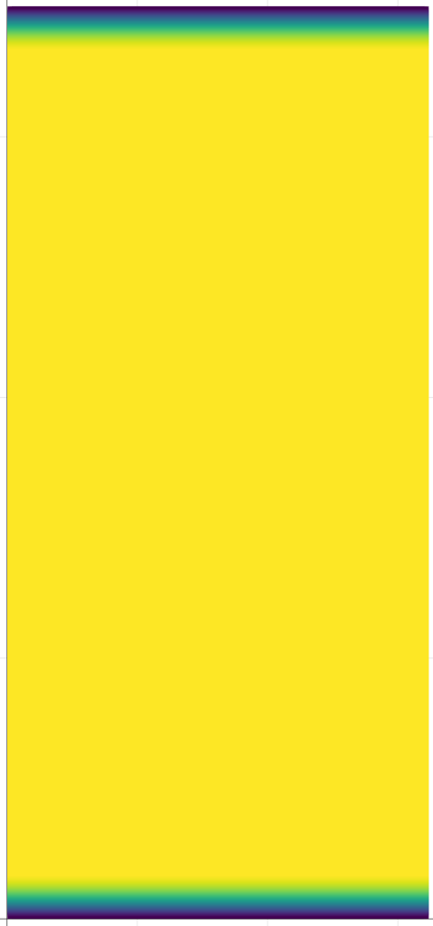
The next step is to incorporate this PML into our material grid. We can simply multiply the S matrix into the material matrices as before, or just multiply and divide the corresponding s entries as follows
μ_r_x = μ_r_2X_Grid ./ sx .* sy
μ_r_y = μ_r_2X_Grid .* sx ./ sy
μ_r_z = μ_r_2X_Grid .* sx .* sy
e_r_x = e_r_2X_Grid ./ sx .* sy
e_r_y = e_r_2X_Grid .* sx ./ sy
e_r_z = e_r_2X_Grid .* sx .* sy
Setting up Ax=B
Combining everything we have solved for so far, we now need to construct our A matrix. We calculate the derivative matrices as before
DEX,DEY,DHX,DHY = yee_grid_derivative(NGRID,k₀*RES, thisBC, k_inc/k₀) # Normalize k termsWe make our material matrices as diagonal matrices to match the dimensionality of the derivative matrices. In this case, because it is only a diagonal, we store these as sparse matrices.
e_r_x = spdiagm(0 => e_r_x[:])
e_r_y = spdiagm(0 => e_r_y[:])
e_r_z = spdiagm(0 => e_r_z[:])
μ_r_z = spdiagm(0 => μ_r_z[:])
μ_r_x = spdiagm(0 => μ_r_x[:])
μ_r_y = spdiagm(0 => μ_r_y[:])
We can then solve for A by incorporating these derivative matrices with the material matrices as defined by the mode of the solution we want to solve for.
if Polarization == H
    A = DHX/μ_r_y*DEX + DHY/μ_r_x*DEY + e_r_z
elseif Polarization == E
    A = DEX/ϵ_r_y*DHX + DEY/ϵ_r_x*DHY + μ_r_z
end
Next we need b. As the trivial solution to Ax=b if b = 0 is just x = 0, we need a better choice of b. Obviously, we want to illuminate our device with a plane wave of some sort. We can simulate a plane wave source by first creating a plane wave in the entire solution space. This solution has a skew excitation at 15 degrees.
F_Src = [exp(1.0im*-(k_inc[1]*i + k_inc[2]*j)) for i = 1:NGRID[1], j = 1:NGRID[2]]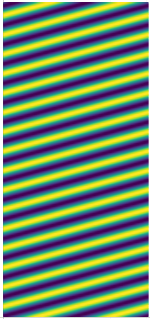
The next part is kinda tricky. Dr, Raymond Rumpf who helped me with this project developed a method of adding an excitation to the solution space while still satisfying Maxwell's aligneds. He called it a total field/scattered field problem Rumpf_2012 . We first set a mask for where we want to seperate total field from scattered field. This is called a Q matrix. It is generally a good idea to place this in the free space between the PML and the device.


By solving the following, we can generate an excitation b that satisfies Maxwell's aligneds. This is true because it generates a b that exists only at the interface between the total field and the scattered field. A more detailed summary of this formulation is in his paper.
$$\begin{aligned} b = (QA - AQ)*f \end{aligned}$$If there was no device, there would simply by the source excitation beneath this boundary and zeros above.
Solvers
Finally, we have an Ax=b to solve! The problem though is that the matrices we made, if they were not sparse, are over 900 million entries. Any significant amount of resolution would require enormous amounts of RAM to solve. The solutions presented here are solved directly, although an iterative solver could be used.
Last but not least, we ask Julia to solve Ax=b. We have to call Array(A) to convert it to a full array as we previously manipulated it as a sparse matrix.
f = Array(A)\bPost Processing
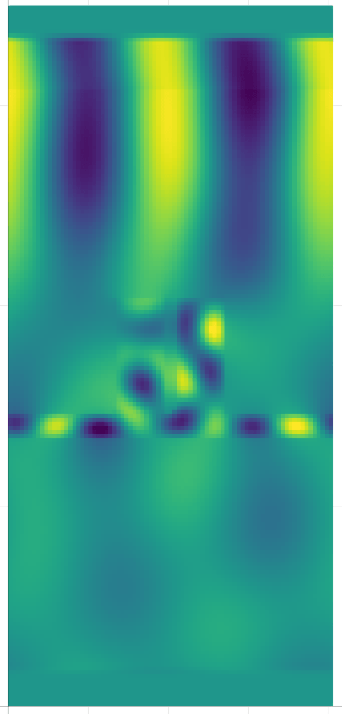
I did not get the chance to perform any calculations of the solved results, but the real part of electric field is as expected.
Future Work
GPU Implementation
One of the interesting things about the finite difference frequency domain problem, is that it can be readily parallelized. Normal CPUs have 4, maybe 8 cores, but graphics cards have hundreds, if not thousands of cores. These cores, however, are made for single instructions but multiple data, SIMD. This is where an iterative solver would really help. We can iterative on several cores at once and converge on a result faster. There are lots of places where the math presented could be sped up with GPUs.
3D Grid and Geometry Voxelization
All of the work presented this far is a 2D simplification of the FDFD problem. This situation is perfectly suited for devices like the presented binary diffraction grating, but the math works in 3D of course. I originally wanted to simulate a volumetric lens antenna in 3D and I wrote a voxelization script for the purpose of parsing 3D geometry into a Yee Grid. That code can be found on the Github of this project.
Final Remarks
All in all, I am very satisfied with the performance of this solver. For 900 million entries, the Julia script solved the problem in 49.9 seconds! Not only that, but the translation from the theory to Julia didn't depend on any crazy syntax. I am excited to see where Julia is going and I hope to expand this code to make use of the most features as possible. The code for this entire project can by found on my Github.
Bibliography
Regier, Miller, McAuliffe, Adams, Hoffman, Lang, Schlegel & Prabhat, Celeste: Variational Inference for a Generative Model of Astronomical Images, 2095-2103, in in: Proceedings of the 32Nd International Conference on International Conference on Machine Learning - Volume 37, edited by JMLR.org (2015) ↩
Kane Yee, Numerical solution of initial boundary value problems involving maxwell’s equations in isotropic media, IEEE Transactions on Antennas and Propagation, 14(3), 302–307 (1966). link. doi. ↩
Sacks, Kingsland, Lee & Jin-Fa Lee, A perfectly matched anisotropic absorber for use as an absorbing boundary condition, IEEE Transactions on Antennas and Propagation, 43(12), 1460–1463 (1995). link. doi. ↩
Rumpf, SIMPLE IMPLEMENTATION OF ARBITRARILY SHAPED TOTAL-FIELD/SCATTERED-FIELD REGIONS IN FINITE-DIFFERENCE FREQUENCY-DOMAIN, Progress In Electromagnetics Research B, 36, 221–248 (2012). link. doi. ↩
Special Thanks
A quick special thanks to Dr. Raymond Rumpf from the University of Texas El Paso for helping me understand the FDFD method. He has provided slides and lecture notes from his website as well as support via email on this project. Without him, I would have never been able to get this working!